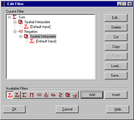
The "Filter" speed button is the fifth (and last) of the Configuration speed buttons. Click on it to reveal the "Edit Filter" frame, and the "Current Filter" window, which is empty. To fill this window, go to the "Available Filters" menu, choose the "Sum" filter (the large sigma icon), and "Add" it.
Click on the "Spatial Interpolate" filter (the overlapping rectangles icon), and Add it.
Illuminate "Spatial Interpolate" in the Current Filter window by left-clicking on it. Then choose the "Default Input" (the red "Zin" icon) filter, and Add it.
Left-click on Sum, and Add the "Negation" filter (the "-f(z)" icon).
Left-click on Negation (in the Current Filter window), and Add Spatial Interpolate.
Illuminate Spatial Interpolate, and Add the Default Input.
Your result should look like this:
Now, we are going to specify the first Spatial Interpolator. Go to it in the Current Filter window, and illuminate it by left-clicking.
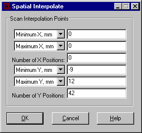
Go to the "Edit" menu item, and click on it to reveal the "Spatial Interpolate" frame, where we will enter "Scan Interpolation Points."
Choose "Minimum Y"=-9, "Maximum Y"=12, "Number of Y Positions"=42. This gives the total scan interval of the leading bobbin coil of the differential-bobbin pair.
Click "OK."
You have returned to the Edit Filter frame, with its Current Filter window. In this window, illuminate the second Spatial Interpolator, by left-clicking on it. Then click on the Edit menu button.
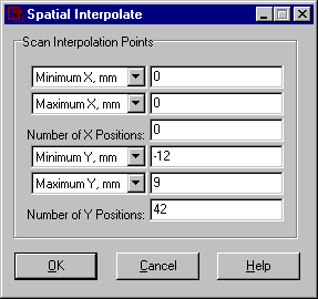
Choose "Minimum Y"=-12, "Maximum Y"=9, "Number of Y Positions"=42. This gives the total scan interval of the trailing bobbin coil of the differential-bobbin pair.
Click OK.
You have just completed defining the differential-bobbin filter, and are now
ready to filter the single-bobbin data through it.
Return to the main VIC-3D® frame, and click on "Apply Filter." This is the third of the "Analyze" speed buttons. A new problem configuration appears, containing the data that resulted from the application of the filter on the original data.