The "2D Plot" plot option, which is exercised through the fourth of the "Analyze" speed-buttons (whose icon contains red and blue wiggly lines), will create plots whose X-axis points are the data in the first column of the data-display window, and whose Y-axis points are the data in the second column.
These columns can be easily exchanged, or otherwise moved, by left-clicking on the header of any column, and then dragging that column to the column which is to be exchanged for it. This allows you to determine the X- and Y-axis data.
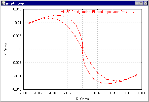
In order to plot the differential-bobbin data in the form of the classical Lissajous figure, click on the first column, "Cylindrical Z," and drag it to the third column, "X."
You have just rearranged the columns, so that "R" is first and "X" second ("Cylindrical Z" is third).
Click on the 2D Plot speed-button. Your result should look like this:
Now, here is an exercise for you. Set up and run a problem that is identical to the one we just analyzed, except that the OD flaw is now only 0.45mm deep, and the number of cells in the depth direction, Nz, is equal to four. An easy way to do this is to save the original problem configuration file under a different name, then make the required changes to the newly-named problem. You'll have to change the boundary location between layers 3 and 4, the flaw R position, and the block depth, in order to properly modify the model. After we run the second problem, we are going to plot its results against our first one, in order to learn the effects of slot-depth on the Lissajous figure.
After the new configuration has been run, apply the same differential-bobbin filter as before. Before plotting the results, be sure that you have given each filtered result a unique descriptive note. Our first one is: "Flaw 1: OD Axial Notch," and the second is "Flaw 2: OD Axial Notch." These notes are printed in the legends of the plots, and will help us interpret the plotted curves.
Go into the Options menu in the main menu bar, and select "Plot Options." Under "Curve and Window Options," check the first one, "Get curve data from all open configurations with similar data arrangements."
Close all windows, except those that carry the filtered data. Unless you have saved them under different names, the latter windows will carry the title "New VIC-3D Configuration (number)"
Once again, be sure to arrange the columns of data in both filtered problems so that resistance (R) is first, reactance (X) is second, and position is third. Click on the 2D Plot icon, and get the following picture:
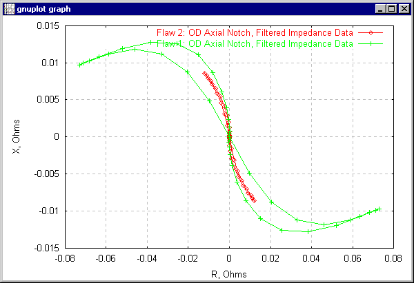
Notice that the shallower slot has a response that is smaller in total extent, and much narrower.